Figure 2A
First compute for shape parameter \(a=0.248\), \(a=1\), \(a=2\) and \(a=15\) the respective scale parameter \(b\) such that the overall connection probability equals \(\mu = 0.1\).
Then we get the relative occurrence of bidirectionally connected pairs \(\varrho\) via
The probability density function fT was defined gamma_functions and is explained in the previous section.
import pylab as pl
import numpy as np

from scipy.optimize import brentq
import scipy.integrate as integrate
from scipy.stats import gamma

from gamma_functions import K, fT


# for different values of a, determine b such that \mu = 0.1
mu = 0.1

def root_f(b):
    return integrate.quad(lambda x: x*fT(x,a,b),0,1)[0] - mu

a_ns = [0.248,1.,2.,15.]
b_ns = [brentq(root_f, 0.5*mu/a, 5*mu/a) for a in a_ns]


# for a,b pairing get the relative overrepresentation \rho
def get_rho(a,b):
    numer = integrate.quad(lambda x:x**2*fT(x,a,b),0,1)[0]
    denom = (integrate.quad(lambda x: x*fT(x,a,b), 0,1)[0])**2
    return numer/denom

rhos = [get_rho(a,b) for a,b in zip(a_ns, b_ns)]

print "a_ns: ", a_ns
print "b_ns: ", b_ns
print "rhos: ", rhos
With this we can create the graphic
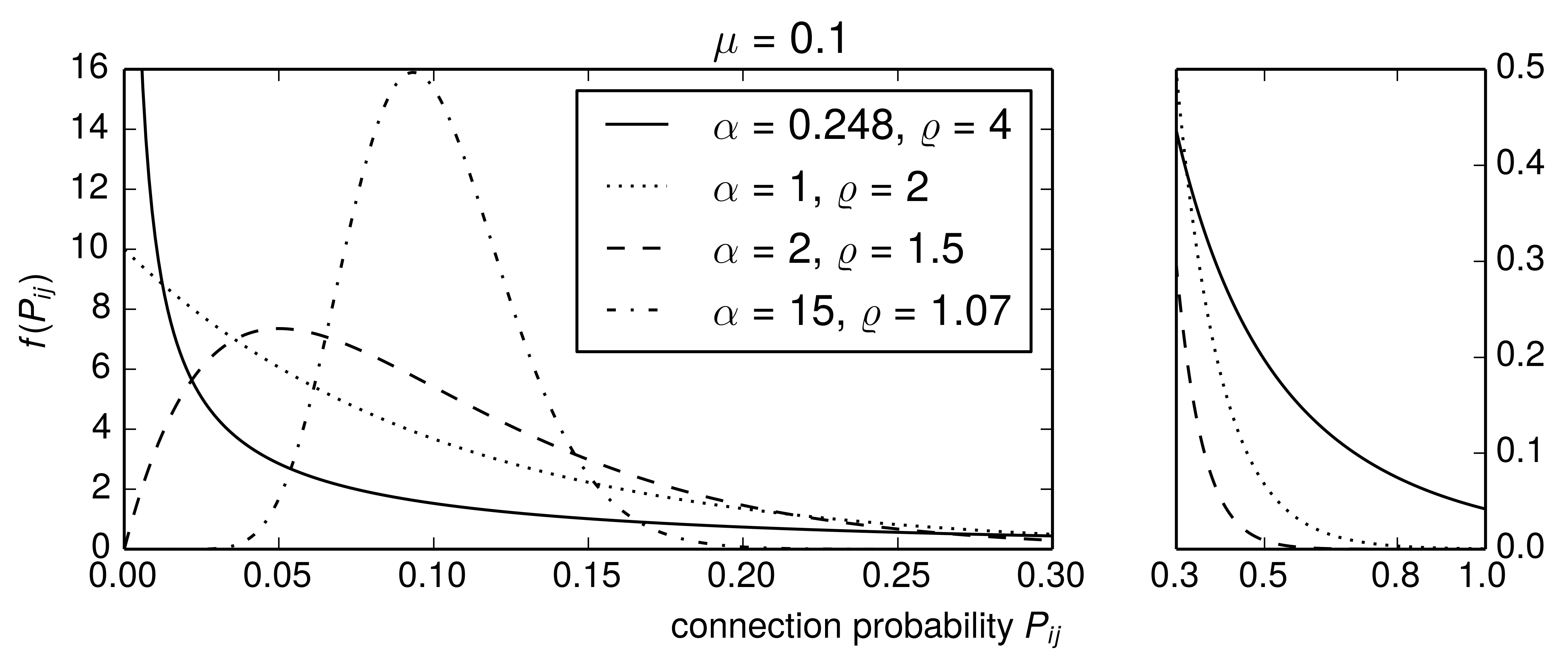
by plotting the probability density functions for the \(a,b, \varrho\) pairings. We can use gamma.pdf from the scipy.stats and only have to scale it by K(a,b) to get the density function for the truncated version.
from matplotlib import rc
from matplotlib import gridspec

rc('text', usetex=True)
pl.rcParams['text.latex.preamble'] = [
    r'\usepackage{tgheros}',    # helvetica font
    r'\usepackage{sansmath}',   # math-font matching  helvetica
    r'\sansmath'                # actually tell tex to use it!
    r'\usepackage{siunitx}',    # micro symbols
    r'\sisetup{detect-all}',    # force siunitx to use the fonts
]


fig, ax = pl.subplots(1,1)
fig.set_size_inches(8.2,2.8)

fig.suptitle(r'$\mu = 0.1$', fontsize=15)

gs = gridspec.GridSpec(1,2, width_ratios = [3,1])
ax_left = pl.subplot(gs[0])
ax_right = pl.subplot(gs[1])

x = np.arange(0,1.+0.001, 0.001)

linestyles = ['-',':','--','-.']

for a,b,rho,ls in zip(a_ns, b_ns,rhos,linestyles):

    # quick sanity check
    h = integrate.quad(lambda z: K(a,b)*gamma.pdf(z, a, scale=b),0,1.)[0]
    assert abs(1.-h) < 10e-6

    ax_left.plot(x, K(a,b)*gamma.pdf(x, a, scale=b),
             'k', label=r'$\alpha = %g$, $\varrho = %.3g$' %(a, rho),
             linestyle=ls)


ax_left.set_xlim(0,0.3)
ax_left.set_ylim(0,16)
ax_left.legend()

label = ax_left.set_xlabel(r'connection probability $P_{ij}$')
ax_left.xaxis.set_label_coords(0.8, -0.135)
ax_left.set_ylabel(r'$f(P_{ij})$')


for a,b,rho,ls in zip(a_ns, b_ns,rhos,linestyles):

    ax_right.plot(x, gamma.pdf(x, a, scale=b), 'k', linestyle=ls)

ax_right.set_xlim(0.3,1.0)
ax_right.set_ylim(0,0.5)

ax_right.set_xticks([0.3, 0.5, 0.8, 1.0])
ax_right.set_yticks([0., 0.1, 0.2, 0.3,0.4, 0.5])

ax_right.yaxis.tick_right()

pl.savefig('gamma_figure_A.pdf', dpi=600, bbox_inches='tight')