Fig 1B
The contour plot
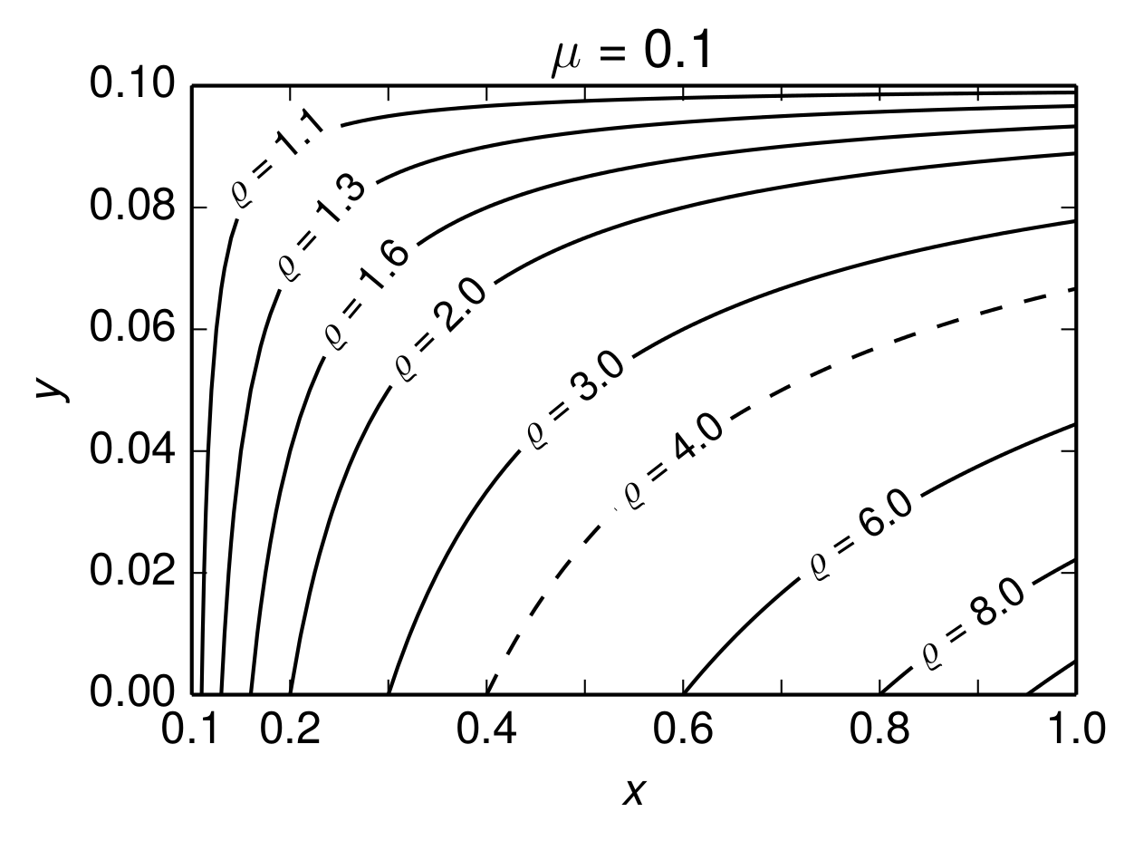
was created using the following Python code
import pylab as pl
import numpy as np

from matplotlib import rc

rc('text', usetex=True)
pl.rcParams['text.latex.preamble'] = [
    r'\usepackage{tgheros}',    # helvetica font
    r'\usepackage{sansmath}',   # math-font matching helvetica
    r'\sansmath'                # actually tell tex to use it!
    r'\usepackage{siunitx}',    # micro symbols
    r'\sisetup{detect-all}',    # force siunitx to use the fonts
]


rhos = [1.1, 1.3, 1.6, 2.0, 3.0, 4.0, 6.0, 8.0, 9.5]
mu = 0.1

s=0.01

xs = np.arange(mu+s, 1.+s , s)
ys = np.arange(0. , 0.1+s, s)

X,Y = np.meshgrid(xs,ys)

curves = (X+Y)/mu - (X*Y)/mu**2

fig = pl.figure()
fig.set_size_inches(4.2,2.8)
ax = fig.add_subplot(111)

manual_locations = [(0.15,0.095), (0.22,0.078), (0.28,0.065),
                    (0.35,0.06), (0.48,0.05), (0.58,0.04),
                    (0.78,0.026), (0.9,0.01) ]

CS = ax.contour(X,Y, curves, rhos,
                colors='k', linestyles=['solid']*5+['dashed'])

ax.clabel(CS, fontsize=11, inline=1,
          fmt=r'$\varrho$ = %1.1f', manual=manual_locations)

pl.ylabel(r'$y$')
pl.xlabel(r'$x$')
pl.xticks(list(pl.xticks()[0]) + [0.1],
          ['0.1','0.2','','0.4','','0.6','','0.8','','1.0'])


pl.title(r'$\mu = 0.1$')

pl.savefig('contour_plot.pdf', dpi=600, bbox_inches='tight')
Here, the expression for curves was used that is stated in the article and was derived in the article's supplementary materials.