Figure 3A
In the generalized model the conditional density function is computed as
where \(N_{\sigma}(x)\) ensures that \(f_{P_{ji}|P_{ij}} (y \mid x)\) integrates to one,
%
Figure 3A shows by the example of the gamma distribution \(f^T_{\alpha,\beta}\) of Figure 2 how \(\sigma\) influences the shape of \(f_{P_{ji} | P_{ij}} (y \mid x)\):
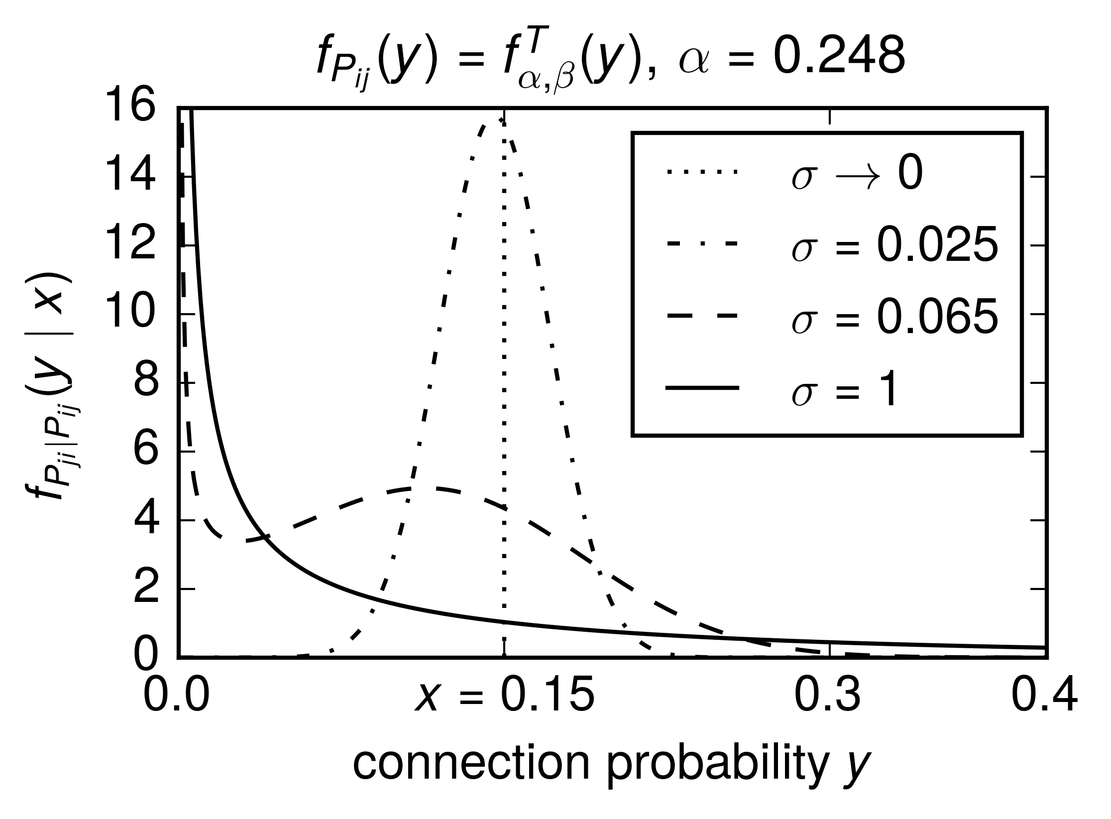
The figure is produced by the following code, requiring the gamma_functions from section K(a,b).
import matplotlib as mpl
mpl.use('Agg')
import pylab as pl

import numpy as np
from gamma_functions import fT, K

from scipy import integrate
from scipy.stats import norm

from matplotlib import rc

rc('text', usetex=True)
pl.rcParams['text.latex.preamble'] = [
    r'\usepackage{tgheros}',    # helvetica font
    r'\usepackage{sansmath}',   # math-font matching  helvetica
    r'\sansmath'                # actually tell tex to use it!
    r'\usepackage{siunitx}',    # micro symbols
    r'\sisetup{detect-all}',    # force siunitx to use the fonts
]


def gamma_sig_graph(alph, bet, xloc, sig):
    '''
    return graph of f^T_{\alpha,\beta}(y)
    ----
    alph : shape parameter alpha
    bet  : scale parameter beta
    xloc : already determined probability x
    sig  : width of modulating normal distribution
    '''

    ys      = np.arange(0,1.+0.001, 0.001)
    fT_vals = []

    # compute normalization factor only once
    Nf = integrate.quad(lambda s: fT(s,alph,bet)
                         *norm.pdf(s,loc=xloc, scale=sig),0,1)[0]

    for y in ys:
        fT_vals.append(fT(y, alph, bet)
                       *norm.pdf(y,loc=xloc,scale=sig)/Nf)

    return ys, fT_vals


fig, ax = pl.subplots(1,1)
fig.set_size_inches(7.5*0.5,2.3)

# from Figure 2
a_ns =  [0.248, 1.0, 2.0, 15.0]
b_ns =  [0.486852833106356, 0.10004560945459162,
         0.0500000206118813, 0.006666666666666667]

alph = a_ns[0]
bet  = b_ns[0]
xloc = 0.15


ax.axvline(x=0.15, ymin=0., ymax=16., color='k', linestyle=":",
           label=r'$\sigma \to 0$')
ax.plot(*gamma_sig_graph(alph,bet,xloc, 0.025),
        'k', linestyle='-.', label=r'$\sigma = 0.025$')
ax.plot(*gamma_sig_graph(alph,bet,xloc, 0.065),
        'k', linestyle='--', label=r'$\sigma = 0.065$')
ax.plot(*gamma_sig_graph(alph,bet,xloc, 1.),
        'k', linestyle='-', label=r'$\sigma = 1$')

ax.set_ylim(0,16)
ax.set_xlim(0,0.4)

pl.xticks([0.,0.15,0.3,0.4], ['0.0', r'$x=0.15$', '0.3','0.4'])
ax.set_title(r'$f_{P_{ij}}(y) = f_{\alpha,\beta}^T(y),\, \alpha=0.248$',
             size=13.)

ax.set_ylabel(r'$f_{P_{ji} | P_{ij}}(y \mid x)$')
ax.set_xlabel(r'connection probability $y$')

pl.legend(prop={'size':12})

pl.savefig('fig3A.pdf', dpi=600, bbox_inches='tight')