Figure 3B
In the generalized model, the relative occurrence of bidirectional connections \(\varrho\) depends on the width \(\sigma\) of the modulating normal distribution.
It is
where \(\operatorname{\mathbf{E}}(P_{ij} P_{ji})\) is computed as the integral
in which the conditional density function is defined as
with normalizing factor \(N_{\sigma}(x)^{-1}\) that makes sure that \(f_{P_{ji}|P_{ij}} (y \mid x)\) integrates to one,
The overall connection probability \(\mu\) is computed as
Generating the data
We generate the data to show this relationship at the example of the gamma distribution (Figure 2) in three different ways:
Numerical integration
In the numerical integration, using scipy.integrate.quad and scipy.integrate.dblquad, the above equations are solved for the given probability density function \(f_{P_{ij}}(y)\) and with \(\sigma\).
import numpy as np

from scipy import integrate
from scipy.optimize import brentq
from scipy.stats import norm

from gamma_functions import K, fT


class Gamma_network(object):

    def __init__(self, a, mu):

        self.a = a
        self.mu = mu

        self.b = self.get_b()

        self.sigma = 1.


    def get_b(self):

        root_f = lambda b: integrate.quad(
            lambda x: x*fT(x,self.a,b),0,1)[0] - self.mu

        return brentq(root_f, 0.5*self.mu/self.a, 5*self.mu/self.a)


    def xyfxfye2(self,x,y):
        numer =  x*y*fT(x,self.a,self.b)*fT(y,self.a,self.b)\
                 *norm.pdf(y,loc=x, scale=self.sigma)
        denom =  integrate.quad(lambda y: fT(y,self.a,self.b)\
                                * norm.pdf(y,loc=x, scale=self.sigma),
                                0,1)[0]
        return numer/denom


    def yfxfye2(self,x,y):
        numer =  y*fT(x,self.a,self.b)*fT(y,self.a,self.b)\
                 *norm.pdf(y,loc=x, scale=self.sigma)
        denom =  integrate.quad(lambda y: fT(y,self.a,self.b)\
                                *norm.pdf(y,loc=x, scale=self.sigma)
                                ,0,1)[0]
        return numer/denom


    def sim(self,sigma):

        self.sigma = sigma

        numer = integrate.dblquad(self.xyfxfye2, 0, 1,
                                  lambda x: 0, lambda x: 1)[0]
        denom_x = integrate.quad(lambda x: x*fT(x,self.a,self.b), 0,1)[0]
        denom_y = integrate.dblquad(self.yfxfye2, 0, 1,
                                    lambda x: 0, lambda x: 1)[0]
        return numer, denom_x, denom_y
Then to get the data, for example for \(\alpha=1\), the following code is executed saving every data point as a dictionary item for full transparency and reproducibility.
if __name__=="__main__":

    import os, pickle

    label = "th_a1_mu01.p"

    gn = Gamma_network(1, 0.1)
    data_frame = []

    with open("data/" + label, "wb") as pfile:
        pickle.dump(data_frame, pfile)

    for sigma in np.arange(0.005,0.75005,0.005):

        numer, denom_x, denom_y  = gn.sim(sigma)
        print( sigma )
        print( "\t numer       : ", numer )
        print( "\t den_x, den_y: ", denom_x, ", ", denom_y )
        print( "\t rho         : ", numer/(denom_x*denom_y) )
        print( "\t alph, bet   : ", gn.a, ", ", gn.b )

        data = {}
        data["alpha"] = gn.a
        data["beta"] = gn.b
        data["mu"] = gn.mu
        data["sigma"] = sigma
        data["numer"] = numer
        data["den_x"] = denom_x
        data["den_y"] = denom_y

        data_frame.append(data)

        os.rename("data/" + label, "tmp/" + label)
        with open("data/" + label, "wb") as pfile:
            pickle.dump(data_frame, pfile)
Sampling of connection probabilities
The numerical integration becomes very resource demanding for specific distributions. In these situations we connection probabilities from the random variables and compute the mean overrepresentation \(\varrho\). To define random variables with the desired distributions scipy.stats.rv_continuous is used.
import numpy as np
from scipy.stats import norm
from scipy.stats import rv_continuous
from scipy.special import gamma
import scipy.integrate as integrate
from scipy.optimize import brentq

from gamma_functions import fT,K


class Rv_Mult_Norm(rv_continuous):

    def __init__(self, rv, x, sigma):

        self.rv = rv
        self.x = x
        self.sigma = sigma

        self.norm_f = self.compute_norm_f()

        rv_continuous.__init__(self, a=0, b=1)

    def compute_norm_f(self):
        return integrate.quad(lambda y: self.rv.pdf(y)\
                              *norm.pdf(y, loc=self.x, scale=self.sigma),
                              0, 1)[0]

    def _pdf(self, y):
        return self.rv.pdf(y)*norm.pdf(y, loc=self.x, scale=self.sigma)/self.norm_f


def sample_rv_mult_norm(x, rv, sigma):

    rv_mult_norm = Rv_Mult_Norm(rv, x, sigma)

    return rv_mult_norm.rvs()


class Trunc_Gamma_Rv(rv_continuous):

    def __init__(self, alph, bet, mu):

        self.alph = alph
        self.bet = bet
        self.mu = mu

        assert(abs(bet-self.get_b())<0.01)
        self.K_ab = self.get_K()

        rv_continuous.__init__(self, a=0, b=1)

    def get_b(self):
        root_f = lambda bet: integrate.quad(
            lambda x: x*fT(x,self.alph,bet),0,1)[0] - self.mu
        return brentq(root_f, 0.5*self.mu/self.alph, 5*self.mu/self.alph)

    def get_K(self):
        a,b = self.alph, self.bet
        int_f_0_1 = integrate.quad(
            lambda x: 1/(b**a*gamma(a))*x**(a-1)*np.exp(-x/b),0,1)
        K_ab = 1./(int_f_0_1[0])
        return K_ab

    def _pdf(self, x):
        if x < 0:
            fT_ab = 0
        elif x>1:
            fT_ab = 0
        else:
            fT_ab = self.K_ab * 1/(self.bet**self.alph*gamma(self.alph))\
                    *x**(self.alph-1)*np.exp(-x/self.bet)

        return fT_ab
Then to get the data, for example for \(\alpha=0.248\), the following code is executed saving every data point as a dictionary item for full transparency and reproducibility.
if __name__ == '__main__':

    from params.sigma_dep_network_params import *
    import os, pickle

    data_frame = []
    label = "4_alpha_0-05_sigma.p"

    with open("data/" + label, "wb") as pfile:
        pickle.dump(data_frame, pfile)

    for alph, bet in zip(alphas,betas):

        rv = Trunc_Gamma_Rv(alph, bet, mu)

        for sigma in np.arange(sig_low, sig_high, sig_step):

            for k in range(n_trials):

                print("a: ", alph, "\t sigma: ", sigma, "\t No.: ", k+1)

                data = {"alpha": alph, "beta": bet, "mu": mu, "sigma": sigma}

                xs = rv.rvs(size=n_pairs)
                ys = []
                for x in xs:
                    y = sample_rv_mult_norm(x, rv, sigma)
                    ys.append(y)

                data["xs"]=xs
                data["ys"]=np.array(ys)

                data_frame.append(data)

                os.rename("data/" + label, "tmp/" + label)
                with open("data/" + label, "wb") as pfile:
                    pickle.dump(data_frame, pfile)
Computation in generated networks
Finally we also tested this method by generating networks with such defined connection probabilities and extracted the relative overrepresentation \(\varrho\).
from __future__ import print_function

import numpy as np
from scipy.stats import norm
from scipy.stats import rv_continuous

import resource

def populate_triu(P, c_rv):
    '''
    Populates the upper triangle of P with connection probabilities
    sampled from c_rv. P_ij is the probability for a connection from
    node i to node j.
    ----------
    P     :  matrix of connection probabiities
    c_rv  :  randomly returns connection probability
    '''

    rows, cols = np.triu_indices_from(P, k=1)

    for i,j in zip(rows,cols):
        P[i][j] = c_rv.rvs()

    assert(np.max(P)<=1)
    assert(np.min(P)>=0)

    return P


def populate_tril(P, c_rvy, params):
    '''
    Populates the lower triangle of P with connection probabilities
    sampled from c_rv, given the corr_method.
    ----------
    P           :  matrix of connection probabiities
    c_rvy      :  class for sampling correlated connection probabilities
    '''

    rows, cols = np.triu_indices_from(P, k=1)

    for i,j in zip(rows,cols):
        c_rvy.x = P[i][j]
        c_rvy.sigma = params["sigma"]
        c_rvy.norm_f = c_rvy.compute_norm_f()
        P[j][i] = c_rvy.rvs()

    assert(np.max(P)<=1)
    assert(np.min(P)>=0)

    return P


class C_rv_mult_norm(rv_continuous):
    '''
    normal modulated random variable for P_ji given P_ij=x
    and width sigma
    '''

    def __init__(self, c_rv, x, sigma):

        self.c_rv = c_rv
        self.x = x
        self.sigma = sigma

        self.norm_f = self.compute_norm_f()

        rv_continuous.__init__(self, a=0, b=1)

    def compute_norm_f(self):
        return integrate.quad(lambda y: self.c_rv.pdf(y)\
                              *norm.pdf(y, loc=self.x, scale=self.sigma),
                              0, 1)[0]

    def _pdf(self, y):
        return self.c_rv.pdf(y)*1/self.norm_f\
               * norm.pdf(y, loc=self.x, scale=self.sigma)


def connect_network(P):

    rel = np.random.uniform(size=np.shape(P))

    return (P>rel).astype(int)


def generate_network(N, c_rv, params):

    P = np.zeros((N,N))
    P = populate_triu(P, c_rv)
    c_rvy = C_rv_mult_norm(c_rv, 1, params["sigma"])
    P = populate_tril(P, c_rvy, params)
    G = connect_network(P)

    return G

def compute_overrep(G):

    N = len(G)

    U = (G+G.T)[np.triu_indices(N,1)]

    n_recip  = float(len(U[np.where(U==2)]))

    p_bar = np.sum(G)/float((N*(N-1)))
    n_recip_bar = p_bar**2*N*(N-1)/2.

    return n_recip/n_recip_bar
For example, for a=1, we collect the data as follows
if __name__ == '__main__':

    import os, pickle

    from gamma_functions import *

    a = 1.
    mu = 0.1

    c_rv = Trunc_gamma(a, mu)

    N = 250
    trials = 5

    df = []

    label = "a_1_sig_05_set5.p"
    with open("data/" + label, "wb") as pfile:
        pickle.dump(df, pfile)

    for sig in np.arange(0.05, 0.45, 0.05):
        params = {"sigma": sig}
        for i in range(trials):
            data = {}
            G = generate_network(N, c_rv, params)
            rho = compute_overrep(G)
            data["rho"] = rho
            data["sig"] = params["sigma"]
            data["mu"]  = float(np.sum(G))/(N*(N-1))
            data["N"] = len(G)
            data["alpha"] = c_rv.alph
            data["beta"] = c_rv.bet

            df.append(data)

            print( sig )
            print( "\t rho         : ", rho )
            print( "\t mu          : ", float(np.sum(G))/(N*(N-1)))

            os.rename("data/" + label, "tmp/" + label)
            with open("data/" + label, "wb") as pfile:
                pickle.dump(df, pfile)
Plotting the figure
With the above methods we generated data and plotted the figure
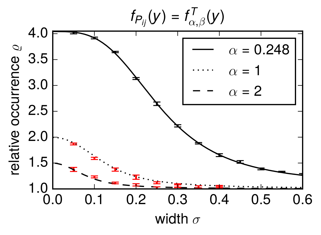
where the red data points were obtained from the generated networks and were not shown in the article. The graphic was created with the following code
import matplotlib as mpl
mpl.use('Agg')
import pylab as pl

import numpy as np
from scipy.stats import sem
import pickle

from matplotlib import rc

rc('text', usetex=True)
pl.rcParams['text.latex.preamble'] = [
    r'\usepackage{tgheros}',    # helvetica font
    r'\usepackage{sansmath}',   # math-font matching helvetica
    r'\sansmath'                # actually tell tex to use it!
    r'\usepackage{siunitx}',    # micro symbols
    r'\sisetup{detect-all}',    # force siunitx to use the fonts
]


# -----  data from numerical integration -----

# a=1
with open("data/th_a1_mu01.p", "rb") as pfile:
    df_a1 = pickle.load(pfile)

# data for sigma=0 from Figure 2
t_sigs_a1 = [0]
t_rhos_a1 = [1.996]

t_sigs_a1 += [d["sigma"] for d in df_a1]
t_rhos_a1 += [d["numer"]/(1./4*(d["den_x"]+d["den_y"])**2) for d in df_a1]

# a=2
with open("data/th_a2_mu01.p", "rb") as pfile:
    df_a2 = pickle.load(pfile)

# data for sigma=0 from Figure
t_sigs_a2 = [0]
t_rhos_a2 = [1.500]

t_sigs_a2 = [d["sigma"] for d in df_a2]
t_rhos_a2 = [d["numer"]/(1./4*(d["den_x"]+d["den_y"])**2) for d in df_a2]


# -----  data from sampling connection probabilities -----

with open("data/4_alpha_0-05_sigma.p", "rb") as pfile:
    df = pickle.load(pfile)

alph = 0.248
x = [d for d in df if d["alpha"]==alph]

sample_sigs = list(set([d["sigma"] for d in x]))
rhos_a0248 = []
rhos_a0248_sem = []

for sigma in sample_sigs:
    df_sig = [d for d in x if d["sigma"]==sigma]
    rhos_sig = [np.mean(d["xs"]*d["ys"])\
                * 1/(np.mean(np.concatenate((d["xs"],d["ys"])))**2)\
                for d in df_sig]
    rhos_a0248.append(np.mean(rhos_sig))
    rhos_a0248_sem.append(sem(rhos_sig))


alph = 1.
x = [d for d in df if d["alpha"]==alph]

sample_sigs_a1 = list(set([d["sigma"] for d in x]))
rhos_a1 = []
rhos_a1_sem = []

for sigma in sample_sigs_a1:
    df_sig = [d for d in x if d["sigma"]==sigma]
    rhos_sig = [np.mean(d["xs"]*d["ys"])\
                * 1/(np.mean(np.concatenate((d["xs"],d["ys"])))**2)\
                for d in df_sig]
    rhos_a1.append(np.mean(rhos_sig))
    rhos_a1_sem.append(sem(rhos_sig))


# ----- fit for alpha=0.248 sampled data -----

xs = np.arange(0.,0.7,0.001)
ys = 1.086317 + (4.043159 - 1.086317)/(1 + (xs/0.2587529)**3.275628)


# ----- data from generated networks -----

# a = 1
with open("data/gn_a1_sig05.p", "rb") as pfile:
    df = pickle.load(pfile, encoding='latin1')

gn_a1_sample_sigs = list(set([d["sig"] for d in df]))

gn_a1_rhos = []
gn_a1_rho_sems = []
for sig in gn_a1_sample_sigs:
    df_sig  = [d for d in df if d["sig"]==sig]
    gn_a1_rhos.append(np.mean([d["rho"] for d in df_sig]))
    gn_a1_rho_sems.append(sem([d["rho"] for d in df_sig]))


# a = 2
with open("data/gn_a2_sig05.p", "rb") as pfile:
    df = pickle.load(pfile, encoding='latin1')

gn_a2_sample_sigs = list(set([d["sig"] for d in df]))

gn_a2_rhos = []
gn_a2_rho_sems = []
for sig in gn_a2_sample_sigs:
    df_sig  = [d for d in df if d["sig"]==sig]
    gn_a2_rhos.append(np.mean([d["rho"] for d in df_sig]))
    gn_a2_rho_sems.append(sem([d["rho"] for d in df_sig]))


fig, ax = pl.subplots(1,1)
fig.set_size_inches(7.5*0.5,2.3)

pl.plot(xs,ys, 'k', label=r'$\alpha=0.248$')
(_, caps, _) = pl.errorbar(sample_sigs, rhos_a0248, yerr=rhos_a0248_sem,
                           fmt="None", ecolor='k', elinewidth=1.5,)
for cap in caps:
    cap.set_markeredgewidth(0.8)

pl.plot(t_sigs_a1, t_rhos_a1, 'k', linestyle=':', label=r'$\alpha=1$')
pl.plot(t_sigs_a2, t_rhos_a2, 'k', linestyle='--', label=r'$\alpha=2$')

(_, caps, _) = pl.errorbar(gn_a1_sample_sigs, gn_a1_rhos, yerr=gn_a1_rho_sems,
                           fmt="None", ecolor = 'r', elinewidth=1.5,)
for cap in caps:
    cap.set_markeredgewidth(0.8)

(_, caps, _) = pl.errorbar(gn_a2_sample_sigs, gn_a2_rhos, yerr=gn_a2_rho_sems,
                           fmt="None", ecolor = 'r', elinewidth=1.5,)
for cap in caps:
    cap.set_markeredgewidth(0.8)

pl.xticks([0.,0.1,0.2,0.3,0.4,0.5,0.6])

ax.set_title(r'$f_{P_{ij}}(y) = f_{\alpha,\beta}^T(y)$', size=13.)
pl.xlim(0,0.6)
pl.ylim(1.,4.05)

pl.legend(prop={'size':12})

pl.xlabel(r'width $\sigma$')
pl.ylabel(r'relative occurrence $\varrho$')

pl.savefig('fig3B.pdf', dpi=600, bbox_inches='tight')